MATLAB Assignment Question And Answer

Introduction Of MATLAB Assignment Question And Answer

This report is used to solve many engineering and computational problems using MATLAB. Paradigms are used to process data, visualise data, develop GUI, and do curve fitting, which may have real-world applications such as material evaluation, power generation analysis, and human motion tracking. A systematic approach silences uncertainties that characterise manual analysis and enhances the accuracy of meaningful results from automated data visualisation.

Need Assignment Help that delivers results? Trusted Assignment Help in UK for well-researched, plagiarism-free academic solutions.

Question 1: Matrix Manipulation

Objective

For processing a force matrix that involves error correction, deletion of rows, and calculation of stiffness based on Hooke’s constant.

Methodology

Extracted the force matrix from assessment_data. mat. Made all values above 100N equal to 0. Copied a matrix and removed two rows. Calculated stiffness = force/depth, and computed mean stiffness (Singh et al., 2022). Identified high stiffness values (≥2× mean) and indexed these. Programmatically computed percentage of high stiffness values.

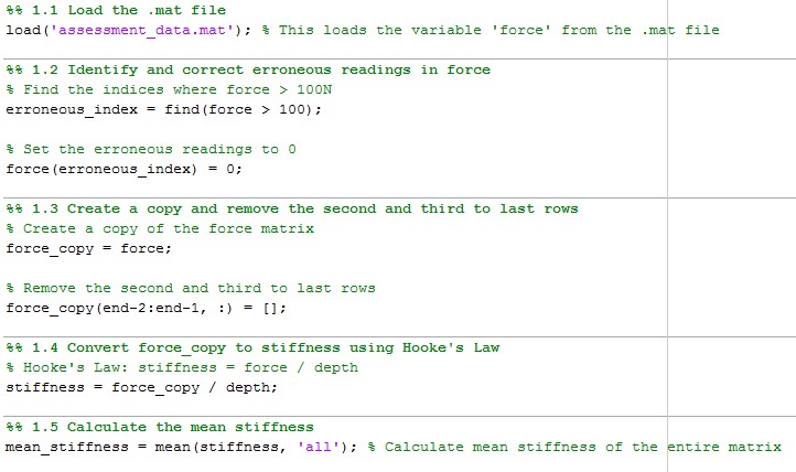
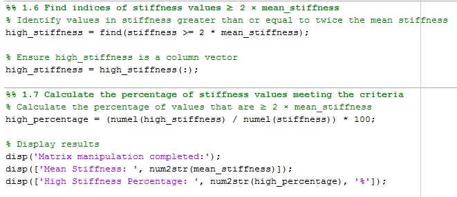
Figure 1: Code for Matrix Manipulation

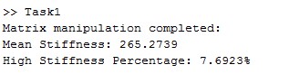
Figure 2: Output

Results

Mean Stiffness: 265.27

High Stiffness Percentage: 7.69%

The task helped to provide proper data processing and further investigation of stiffness properties.

Question 2: File I/O and Plotting

Objective

To filter human motion data and to display the relative hand position and the cumulative distance within a specific period of time.

Figure 3: Code for solving the Question 2

Methodology

The relative hand positions were calculated from the shoulder position obtained from using human_motion_data. csv. A time vector with a sampling rate of 20 Hz was established (Kumar et al., 2021). The total distance reached in the end was determined by using the Euclidean distance formula.

Results

Plots:

1. Relative Hand Position vs. Time:

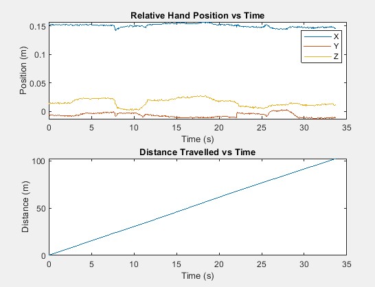
Figure 4: Relative hand positions vs. time

Plots demonstrate placing the X-axis with maximum displacement and equally linear motion during 35 seconds.

1. Distance Traveled vs. Time:

Figure 5: Distance traveled vs Time

The total distance covered by the hand is directly proportional to time, and hence it continues to move throughout the recorded data (Khalil et al., 2020). The total distance covered at the end of 35 seconds is around 100 meters.

Insights

Distance covered is linearly increasing with time, and thus it suggests that the motion is uniform during the entire recording period.

Relative hand position shows that there is variation in motion along different axes. The x-axis is showing the highest movement.

Question 3: Writing Data to File

Objective

In order to write out the processed data for the sample time and relative hand position, they are exported to a tab-separated text file for further analysis and plotting.

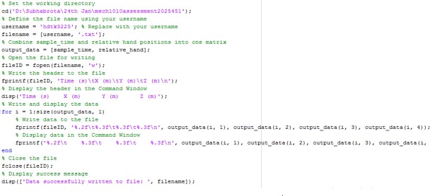
Figure 6: Code for question 3

Methodology

The sample_time and relative_hand matrices were combined into one matrix (Onyibo et al., 2022). A text file named hdtk3225.txt was created with headers: Time (s), X (m), Y (m), and Z (m). Data values were rounded (time: 2 decimal places, positions: 3 decimal places) and written row by row using MATLAB's fprintf function. The same data was displayed in the Command Window for verification.

Results

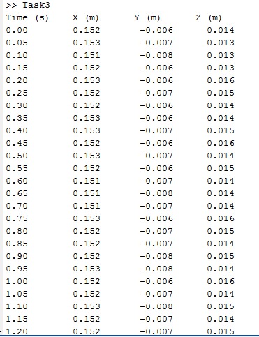
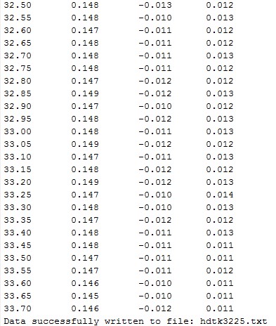
Figure 7: Output

The file hdtk3225.txt was created, which contained data on 4 columns of time and hand position, ranging from 0.00 to 33.70 seconds.

Question 4: Loops and Logic

Objective

In order to detect and remove temperature spikes in a process stream and to compute the heat that must be supplied to heat up a given material downstream.

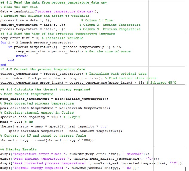
Figure 8: Code for Question 4

Methodology

Process temperature data, which was in the form of process_temperature_data.csv, was used in the analysis for this paper (Zhu et al., 2020). A loop recorded a temperature rise of 45°C at 56 seconds in the process temperature that was subsequently adjusted. Thermal energy was determined from Q=m⋅c⋅ΔT, where mass flow rate m=2.4 kg/min, specific heat c=1800 J/kg °C, and ΔT = mean ambient temperature and peak corrected process temperature. was corrected in the process temperature data.

Results

• Temperature Error Time: 56 seconds
• Mean Ambient Temperature: 22.1063°C
• Peak Corrected Process Temperature: 737.33°C
• Thermal Energy Required: 3090 kJ

Question 5: 3D Plotting and User-defined Functions

Objective
To evaluate water turbine power generation with respect to nozzle and wheel radii and to plot the results in the form of a 3D graph.

Methodology:
Row vectors were used to define wheel radii (0.12–0.30 m) and nozzle radii (0.002–0.010 m). Another loop with the power matrix produced using the waterwheel_generate function was computed for all the radii (Ramseyer et al., 2020). An example was a 3D mesh plot that represented the relationship between the radii and the power production.

Results:

1. 3D Mesh Plot Analysis:

The plot brings out the impacts of nozzle radius, wheel radius, and the power generated. When both radii are started at their most favorable condition, then peak power output is achieved (Raj et al., 2021). The plot shows that, when the nozzle radius goes beyond a certain threshold, the value decreases.

1. Power Matrix Observations:

From the computed power matrix, the highest recorded power out was about 133 W for wheel with a radius of 0.3 m and nozzle with radius of 0.009 m.

Question 6: Curve Fitting and Plotting

Objective
To further compare generator speed and power, fit a second-order polynomial and estimate the power at 225 rpm.

Methodology

Data was extracted from power_speed_curve.txt (the speed of the motor in rad/s and power in milliwatts). Specific speed was obtained by dividing the speed by 3, and a second-order polynomial best fit was used to estimate the speed-power characteristic (Husham et al., 2020). Power at 225 rpm was calculated using the found polynomial. Two plots were created: The first is a comparison of speed (RPM) and power (mW) and the dotted, fitted power curve with the operating point at 225 RPM indicated.

Results

Operating Power at 225 rpm: 7,562.5 mW. The plotted results agreed well with the dependence of speed and power on each other, which was polynomial, and the trends were well defined.

Plots:

Analyzing the speed vs. power from the original data reveals a progressive common power trend with respect to the speed.

The power curve best fitted to the polynomial relation is also depicted with the operating point located at 225 rpm, expressed as the red circle.

Question 7: Logical Indexing

Objective
To filter passing material samples, determine which of them could pass through the filter with ease, and get the aggregate score of the sample with the highest ranking.

Methodology
The sample_data.csv containing the exemplars was read with readtable. Thirty-two samples were taken from six different tests, and the scores were dumped into a numerical array (Ferrando et al., 2020). The assess_sample function averaged the scores for each sample and then decided how many tests out of six the sample passed with at least 60 percent. Logical indexing processed and restricted the passing samples into another table known as pass_samples. The sample with this maximum score average was determined by applying the max function.

Results

Best Sample: Sample 26

Average Score: 78

The automation approach guarantees accuracy for assessing all material samples.

Question 8: Security Questions

Objective

To take multiple-choice quizzes on the concept in cybersecurity.

Answers

1. C (“Encryption”).
2. B (“A corporate email address”).
3. B (“Data Protection Act 2018”).
4. A (“A method of extracting confidential information”).
5. D (“Phishing”).
6. C (“No further testing”).
7. D (“Viewing confidential data”).
8. D (“Cookies”).

Question 9: GUI Development

Objective

Specifically for designing the GUI in order to enable the analysis of data relating to trainer power and cadence.

Methodology

A GUI was created using MATLAB App Designer having Load Script & Run Script buttons, Cadence vs. Time and Power vs. Time plots, and a text area. The “Load Script” button allows the option to input trainer_power_analysis.m, while the “Run Script” button triggers the file to be run and variable and result visuals to be pulled.

The GUI is able to load scripts, plot data within the created GUI, and display average power values. It has an interactive user interface, which includes MATLAB script for data analysis and data visualization.

Conclusion

The tasks described above prove that MATLAB is universally applicable to data processing, visualization, and GUI. Applying the logical indexing, file operations, curve fitting, and 3D plotting integrated in the project shows that the computational tools are very vital in simplifying the assigned tasks and solving engineering problems.

Reference list

Journals

• Ferrando, M., Causone, F., Hong, T., and Chen, Y., 2020. Urban building energy modeling (UBEM) tools: A state-of-the-art review of bottom-up physics-based approaches. Sustainable Cities and Society, 62, p.102408.
• Husham, S., Mustapha, A., Mostafa, S.A., Al-Obaidi, M.K., Mohammed, M.A., Abdulmaged, A.I., and George, S.T., 2020. Comparative analysis between active contour and Otsu thresholding segmentation algorithms in segmenting brain tumor magnetic resonance imaging. Journal of Information Technology Management, 12 (Special Issue: Deep Learning for Visual Information Analytics and Management), pp. 48-61.
• Khalil, I.U., Ul-Haq, A., Mahmoud, Y., Jalal, M., Aamir, M., Ahsan, M.U., and Mehmood, K., 2020. Comparative analysis of photovoltaic faults and performance evaluation of its detection techniques. IEEE Access, 8, pp. 26676-26700.
• Kumar, A., Krishnamurthi, R., Bhatia, S., Kaushik, K., Ahuja, N.J., Nayyar, A., and Masud, M., 2021. Blended learning tools and practices: A comprehensive analysis. IEEE Access, 9, pp. 85151-85197.
• Onyibo, E.C. and Safaei, B., 2022. Application of finite element analysis to honeycomb sandwich structures: a review. Reports in Mechanical Engineering, 3(1), pp. 192-209.
• Raj, B.P., Meena, C.S., Agarwal, N., Saini, L., Hussain Khahro, S., Subramaniam, U., and Ghosh, A., 2021. A review on the numerical approach to achieve building energy efficiency for energy, economy, and environment (3E) benefits. Energies, 14(15), p.4487.
• Ramseyer, F.T., 2020. Motion energy analysis (MEA): A primer on the assessment of motion from video. Journal of Counseling Psychology, 67(4), p. 536.
• Singh, N., Gunjan, V.K., and Nasralla, M.M., 2022. A parameterized comparative analysis of performance between the proposed adaptive and personalized tutoring system “Seis Tutor” and existing online tutoring systems. IEEE Access, 10, pp.39376-39386.
• Zhu, L., Karim, M.M., Sharif, K., Xu, C., Li, F., Du, X., and Guizani, M., 2020. SDN controllers: A comprehensive analysis and performance evaluation study. ACM Computing Surveys (CSUR), 53(6), pp.1-40.