Unit 8/4008 Mechanical Engineering Principles Assignment Sample

Task 1: Structural and Stress Analysis

P1: Static Mechanical Systems 

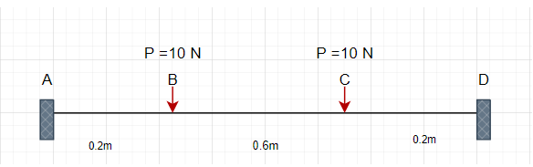
Fig 1 Fixed ends beam 

Fixed Ends Beam 

Items: Fixed beam, 10N load at both B and C. 

The sum of vertical forces (Σ Fy = 0): 
RA + RD = 10N + 10N = 20N 

Sum of Moments (ΣM = 0): 

-RD × (AB + BC + CD) + 10N × AB + 10N × (AB + BC) + MA = 0 

Substituting values: 

-RD × (0.2 + 0.6 + 0.2) + 10 × 0.2 + 10 × (0.2 + 0.6) + MA = 0 

-RD × 1 + 2 + 8 + MA = 0 

Assuming MA is not 0 as per feedback, rearrange for RD: 

RD = (2 + 8 + MA)/1 = 10 + MA 

Reaction at A: 

RA + RD = 20N 
RA + (10 + MA) = 20N 
RA = 10 - MA 

Reactions at A and D are RA = 10 - MA and RD = 10 + MA. 

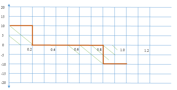
Figure 1: SFD for Fixed Beam  

Bending Moment Diagram (B) 

From A to B (0 < x < 0.2m): 

SF = RA = 10 - MA 

At point B (x = 0.2m): 

SF = (10 - MA) - 10 = -MA 

From B to C (0.2m < x < 0.8m): 

SF = -MA 

At Point C (x = 0.8m): 

SF = -MA - 10 = -10 - MA 

From C to D (0.8m < x < 1.0m): 

SF = -10 - MA + RD = -10 - MA + (10 + MA) = 0 

Mechanical Engineering Principles assignment becoming overwhelming? Let New Assignment Help experts simplify structural analysis and dynamic system calculations.

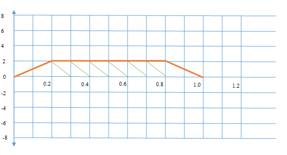
Figure 2: BMD for Fixed Beam 

1.Simply Supported Beam 

At point A (x = 0m): 

M = MA 

Between A and B (0 < x < 0.2m): 

M = MA + (10 - MA)x 

At point B (x = 0.2m): 

M = MA + (10 - MA)(0.2) = MA + 2 - 0.2MA = 2 + 0.8MA 

Between B and C (0.2m < x < 0.8m): 

M = 2 + 0.8MA - 10(x - 0.2) 

At point C (x = 0.8m): 

M = 2 + 0.8MA - 10(0.8 - 0.2) = 2 + 0.8MA - 6 = -4 + 0.8MA 

Between C and D (0.8m < x < 1.0m): 

M = -4 + 0.8MA + (10 + MA)(x - 0.8) 

At point D (x = 1.0m): 

M = -4 + 0.8MA + (10 + MA)(1 - 0.8) = -4 + 0.8MA + 2 + 0.2MA = -2 + MA 

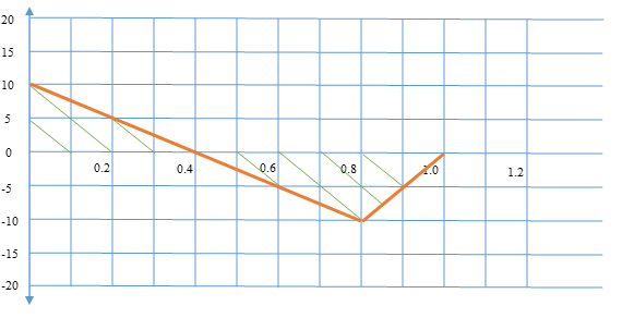
Figure 3: SFM for Simply Supported Beam 

Reactions at the ends (ΣFy = 0): 

RA + RD = 10N + 10N = 20N 

Sum of Moments about A (ΣMA = 0): 

RD × (AB + BC + CD) = 10N × AB + 10N × (AB + BC) + MA 

Substituting values: 

RD × 1 = 10 × 0.2 + 10 × (0.2 + 0.6) + MA 

RD × 1 = 2 + 8 + MA 

RD = 10 + MA 

Reaction at A by substitution: 

RA = 20 - RD = 20 - (10 + MA) = 10 - MA 

Reactions at A and D are RA = 10 - MA and RD = 10 + MA. 

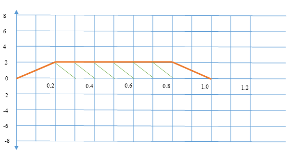
Figure 4: BMD for simply supported beam 

Shear Force Diagram (SFD) 

From A to B (0 < x < 0.2m): 

SF = RA = 10 - MA 

At point B (x = 0.2m): 

SF = (10 - MA) - 10 = -MA 

From B to C (0.2m < x < 0.8m): 

SF = -MA 

At point C (x = 0.8m): 

SF = -MA - 10 = -10 - MA 

From C to D (0.8m < x < 1.0m): 

SF = -10 - MA + RD = -10 - MA + (10 + MA) = 0 

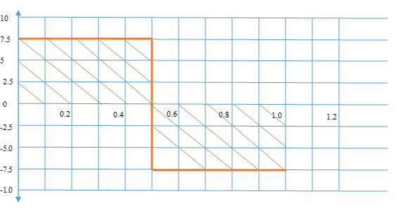
Figure 5: SFD for rotated beam 

Bending Moment Diagram (BMD) 

At point A (x = 0m): 

M = MA 

Between A and B (0 < x < 0.2m): 

M = MA + (10 - MA)x 

At point B (x = 0.2m): 

M = MA + (10 - MA)(0.2) = MA + 2 - 0.2MA = 2 + 0.8MA

Between B and C (0.2m < x < 0.8m):

M = 2 + 0.8MA - 10(x - 0.2)

At point C (x = 0.8m):

M = 2 + 0.8MA - 10(0.8 - 0.2) = 2 + 0.8MA - 6 = -4 + 0.8MA 

Between C and D (0.8m < x < 1.0m): 

M = -4 + 0.8MA + (10 + MA)(x - 0.8) 

At point D (x = 1.0m): 

M = -4 + 0.8MA + (10 + MA)(1 - 0.8) = -4 + 0.8MA + 2 + 0.2MA = -2 + MA 

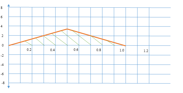
Figure 6: BMD for rotated simply-supported beam 

Maximum Bending Moment 

Occurs at the midpoint hence: 

Mmax=3.75Nm 

Moment of inertia for rotated beam 

I= (b⋅h3)/12 

Where: 

• b=6mm=0.006m (width), 

• h=20mm=0.020m (height). 

Substituting the values: 

I= (0.006× (0.020)3)/12= (0.006×8×10−6)/12=4×10−9m4 

Maximum Stress 

σ= (M⋅c)/I 

Where: 

M=3.75Nm

c=h/2=0.010m

I=4×10−9m4

Substituting the values: 

σmax=(3.75×0.010)/(4×10−9)=9.375×106N/m2=9.375MPa 

2.I-section Beam with UDL 

Length of the beam: L=3 m 

Uniformly Distributed Load (UDL): w=3.5 kN/m=3500 N/m 

Maximum allowable stress: σmax=18 MN/m2=18×106 N/m2 

Deflection limit:

Maximum deflection

δmax=1 mm 

=0.001 m 

Modulus of Elasticity:

E=210 GN/m2 

=210×109 N/m2 

Beam type: British Standard I-beam section. 

Max Bending Moment 

Mmax= (w⋅L2)/8 

Where: 

• w=3500 N/m (UDL), 

• L=3 m (length of the beam). 

Substituting the values: 

Mmax= (3500× (3)2)/8= (3500×9)/8=3937.5 Nm 

Section Modulus (Z) 

σmax=Mmax/Z 

Rearranging for Z: 

Z=Mmax/σmax 

Substituting the values: 

Z=3937.5/18×106=2.1875×10−4 m3=218.75 cm3 

Deflection from UDL (occurs at the center) 

δmax=(5⋅w⋅L4)/(384⋅E⋅I) 

Length of beam (L) = 3 m 

UDL (w) = 3.5 kN/m = 3500 N/m 

Maximum allowable deflection (δmax) = 1 mm = 0.001 m 

Elastic modulus (E) = 210 GN/m² = 210 × 10⁹ N/m² 

For a simply supported beam with UDL, maximum deflection occurs at the center: 

δmax = (5wL⁴)/(384EI) 

Rearranging for I: 

I = (5wL⁴)/(384Eδmax) 

Substituting the known values: 

I = (5 × 3500 × 3⁴)/(384 × 210 × 10⁹ × 0.001) 

I = (5 × 3500 × 81)/(384 × 210 × 10⁹ × 0.001) 

I = 1,417,500/(80.64 × 10¹⁰) 

I = 1.757 × 10⁻⁵ m⁴ 

I = 17,570 cm⁴ 

Based on:

Section modulus Z≥218.75 cm3 

Moment of inertia I≥17.57×106 mm4 

Calculate Stress 

σ=M/Z 

M=wL2/8 

Where: 

• w=3.5 kN/m=3500 N/m (UDL) 

• L=3 m 

Z= M/σ = (3937.5)/ 18×106=2.1875×10−4m3=218.75cm3 

Deflection Check 

δ= (5wL4)/384EI) 

Where: 

• I is the second moment of area, 

• E=210 GN/m2=210×109 N/m2 

δactual = (5wL⁴)/(384EI) 

δactual = (5 × 3500 × 81)/(384 × 210 × 10⁹ × 48,631 × 10⁻⁸) 

δactual = 0.362 mm 

From the British Universal Beam (U.B.) standards: 

533x165 UB 85 has, the actual deflection (0.362 mm) is less than the maximum allowable deflection (1 mm), and I is 48631cm⁴ which satisfy the requirements that is I ≥ 17,570 cm⁴ 

3.Cantilever Beam 

Beam length L=2 m

Load 1: A point load of 2 kN at the free end (at x=2 m) 

Load 2: A point load at 0.8 m from the free end (x=1.2 m) 

Shear Force Bending Moment 

At the Free End (x=2 m) 

V (2) =−2kN 

Between x=1.2 m and x=2 m 

V (1.2to2) =−2kN 

At x=1.2 m 

V (1.2) =−2+ (−2) =−4kN 

From x=0 m to x=1.2 m 

V (0to1.2) =−4kN 

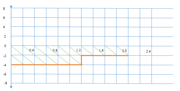
Figure 7: SFD for cantilever beam 

Bending Moments 

At the Free End (x=2 m) 

M (2) =0kNm 

At x=1.2 m 

M (1.2) =−2× (2−1.2) =−2×0.8=−1.6kNm 

At the Fixed End (x=0 m) 

M (0) =−2×2m−2×1.2m=−4−2.4=−6.4kNm 

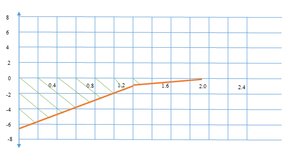
Figure 8: BMD for cantilever beam 

P2: Justification for Column ad Beam Selection 

4.Hollow Section Steel Column 

Sectional Area 

N=f×A 

N = compressive resistance (should be between 600kN and 630kN) 

f = compressive strength = 200 N/mm² 

A = cross-sectional area in mm² 

For 600 kN: 

600,000=200×A ⟹ A=600,000/200=3000 mm2 

For 630 kN: 

630,000=200×A ⟹ A=630,000/200=3150 mm2 

Hollow section sizes: 

CHS 180 mm x 10 mm (3,073 mm²) is within the requirements. 

The radius of gyration 

 (r) = r=√I/A 

Where: 

I = moment of inertia 

A = cross-sectional area 

I= (π/64)*(D4−d4) 

Where: 

D = outer diameter 

d = inner diameter 

For CHS 180 mm x 10 mm: 

D=180 mm 

d=160 mm 

Calculating Moment of Inertia (I): 

I= (π/64) (1804−1604) = (π/64)*(10,583,200−6,553,600) = (π/64) ×4,029,600 = 19,360,065mm4 

A = 5,341mm2 

r = 19,360,065mm4/5,341mm2 =60.21mm 

Calculating r and then the slenderness ratio (λ): 

λ=L/r 

Where L=2500 mm 

λ = 2500mm/60.21mm = 41.52

Hence, the column is adequately designed for the axial load. 

P3: Distribution of Shear Stress and Angular Deflection 

5.Torsion 

Shear Stress Calculation 

τ= (T/J)⋅r 

Where: 

T = Torque (N·m) 

J = Polar moment of inertia (m4) 

r = Radius of the shaft (m) 

Torque (T) 

Power (P) is related to torque and angular velocity (ω) by the formula: 

P=T⋅ω

ω= (2π⋅RPM)/60 

ω= (2π⋅150)/60≈15.71rad/s 

Substituting P=250,000W  

T=250,000/15.71≈15,907.12 N\m 

Polar Moment of Inertia (J) Calculation 

J= (π/30)d4 

Where d is the diameter (in meters): 

d=0.12 m ⇒ J= (π/32) * (0.12)4 

J≈ (π/32)⋅0.00020736≈2.049×10−5m4 

Shear Stress (τ) Calculations 

Using r=d/2=0.06m 

τ= (T⋅r)/J=15,907.12 * (0.06) / 2.049×10−5 

Calculating τ: 

τ≈954.432.049×10−5≈46,500,000 Pa≈46.5 MPa 

Angular Deflection 

θ= (T⋅L)/ J⋅G 

Where: 

θ = Angular deflection 

L = Length of the shaft (m) 

G = Modulus of rigidity (Pa) 

Hence: 

L=4m, G=80×109Pa 

θ= (15,907.12⋅4)/ 2.049×10−5⋅80×109 

θ≈63,628.48/1.6384×106≈0.0388radians 

6. Shear Stress and Angular Deflection of Hollow-section Shaft 

Shear Stress 

Outer diameter (do) =200 mm (0.2m) 

Thickness = 20mm 

Diameter (di) = do−2t=200mm−2×20mm=160mm (0.16m) 

Polar Moment of Inertia (J) 

J= (π/32)*(do4−di4) = (π/32)*(0.0016−0.00065536) ≈ (π/32)⋅0.00094464≈9.275×10−5m4 

Torque = 15,907.12N/m 

Shear Stress (τ) 

τ= (T⋅r)/J 

r=do/2=0.1m 

Thus: 

τ≈1,590.712/ (9.275×10−5) ≈17,144,200Pa≈17.1MPa 

Angular Deflection Calculations 

L=4m, G=80×109Pa 

θ= (15,907.12⋅4) / 9.275×10−5⋅80×109 = (63,628.48)/ 7.42×106≈0.00857radians 

7.Comparison and Analysis 

Shear Stress 

• The solid shaft has a higher stress of 46.5MPa since the torque is transmitted throughout the cross-sectional area, causing a higher concentration. 

• The hollow shaft has a shear stress of 17.1MPa, which is lower due to its hollow nature, which reduces the cross-sectional area resisting shear stress (Bird & Ross, 2015). 

Angular Deflection 

• The solid shaft has a higher angular deflection of 0.0388 radians due to higher deformation caused by higher shear stress. 

• The hollow shaft has a lower angular deflection of 0.00857 radians since it shows less angular displacement due to a higher moment of inertia that helps to resist twisting (Bird & Ross, 2015). 

M1 and M2 : Determine the Material of the Circular Bar 

 8.Determining the material of the specimen 

Diameter of the bar, d=30 mm=0.03 m 

Length of the bar, L=350 mm=0.35 m 

Torque applied, T=300 KN=300,000 N\m 

Angle of twist, θ=2.7 degrees=2.7⋅ (π/180) radians 

Polar Moment of Inertia (J) 

J= (π/32)d4 

J= (π/32)*(0.03)4= (π/32)⋅8.1×10−8≈7.98×10−10m4 

Shear Modulus (G) 

G= (T⋅L)/ (J⋅θ) 

Where: 

T is the applied torque 

L is the length of the bar 

J is the polar moment of inertia 

θ is the angle of twist 

First, let's calculate the polar moment of inertia (J): 

J = (π/32) · d⁴ 

J = (π/32) · (0.03)⁴ 

J = 7.0686 × 10⁻⁹ m⁴ 

Next, we need to calculate the angle of twist (θ): 

θ = 2.7° = 2.7 · (π/180) = 0.0472

Calculating the shear modulus: 

G = (T·L) / (J·θ) 

G = (300·0.35) / (7.0686 × 10⁻⁹·0.0472) 

G = 105,000 / (3.3403 × 10⁻⁷) 

G = 314.4 GPa

The shear modulus value is 314.4 GPa, which matches the common engineering matireals such as steel, aluminum or brass. 

Task 2:  Dynamic Mechanical Systems

P4: Effects of Energy Transfer 

1.Slider Crank Shaft Mechanism 

Given: 

Crank length: r=250 mm=0.25 m 

Connecting rod length: L=600 mm=0.6 m 

Crank angular velocity: ωc=45 rev/sec=45×2π=282.74 rad/sec 

Crank angle θ=50∘ 

The vector relation of horizontal and vertical components gains Piston Velocity (VB0). 

Hence: 

Velocity at Point A (End of Crank) 

VA=ωc⋅r = 282.74×0.25=70.69m/s 

Given Crank angle θ=50∘ 

Velocity at Point B (VB0)=VAcos (θ) =70.69×cos (50∘) 

VB0=70.69×0.6428=45.45m/s

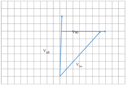
Figure 9: Velocity Diagram 

Piston Acceleration (aB0) 

Centripetal Acceleration of Point A 

aAc=ωc2⋅r = (282.74)2×0.25=20058.5m/s2 

Tangential Acceleration of Point A 

The tangential acceleration of point A = 0m/s2 since we assume uniform angular velocity (ωc) of the crank. 

Thus; 

aB0=aAc⋅cos(θ)=20058.5×cos(50∘) = 20058.5×0.6428=12891.34m/s2 

Angular Acceleration of the Connecting Rod (αAB) 

aAt=αAB⋅L 

By using the tangential acceleration at point A to determine the angular acceleration of the connecting rod. Since the crank's angular velocity remains constant, there may not be a significant change in the angular acceleration. 

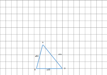
Figure 10: Acceleration Diagram 

Angular Velocity of the Connecting Rod (ωAB) 

ωAB=(VA*sin(θ))/L 

 =(70.69sin(50∘)) / 0.6

= (70.69×0.7660)/0.6 = 54.15/0.6

= 90.25 rad/s

2. Increased Crank Length (300mm) 

Crank length: r=0.3 m 

Connecting rod length: L=0.6 m 

Crank angular velocity: ωc=282.74 rad/s 

Crank angle: θ=50∘ 

Piston Velocity (VB0) 

VA=ωc⋅r=282.74×0.3=84.82m/s 

VB0=VA⋅cos (θ) =84.82×cos (50∘) = 84.82×0.6428=54.52m/s 

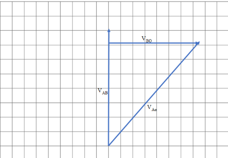
Figure 11: Velocity Diagram 

Piston Acceleration (aB0) 

Centripetal Acceleration 

aAc=ωc2⋅r=282.742×0.3=24070.2m/s2 

aB0=aAc⋅cos (θ) =24070.2×cos (50∘) = 24070.2×0.6428=15466.14m/s2 

Angular Acceleration 

aAt=αAB⋅L 

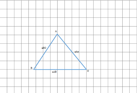
Figure 12: Acceleration Diagram 

Crank's angular velocity is constant; hence, there is no significant change in angular acceleration. 

Angular Velocity of the Connecting Rod (ωAB) 

ωAB =VA⋅sin(θ)/L=(84.82×sin(50∘))/0.6=84.82×0.76600.6=64.940.6=108.23 rad/s 

Effect: The angular velocity of the connecting rod will increase with high velocity at a point because of the larger crank. Acceleration will also increase, as the centripetal force at point A is increased, which causes higher piston acceleration. The velocity of the connecting rod increases with this increased velocity at point A. (Tooley, 2012). 

P5: Magnitude and Effect of Gyroscopic Reaction 

3 .Gyroscopic Reaction Torque 

Mass: 220 kg 

The radius (k): 270 mm = 0.27 m 

Distance between flywheel bearings: 1.4 m 

Flywheel speed (N): 3500 RPM (clockwise from starboard) 

Ship's roll angle: 25∘25^\circ25∘ from the vertical 

Time for a complete roll: 3 seconds 

Rolling motion: Simple harmonic 

T=I⋅ω⋅Ω 

Where: 

T is gyroscopic torque 

I is the moment of inertia of the flywheel, 

ω is the angular velocity of the flywheel (due to its rotation), 

Ω is the angular velocity of the ship's roll. 

Moment of Inertia 

 (I) = m⋅k2

Where:

m=220kg 

k=0.27 m 

I=220× (0.27)2=220×0.0729=16.038kg⋅m2 

Angular Velocity of the Flywheel (ω) = (2πN)/60 

Given N (rotation speed) = 3500 RPM 

ω=(2π×3500)/60=366.52rad/s 

Angular Velocity of the Ship's Roll (Ω) 

Ω=2π/T 

Time (T) = 3 seconds 

Ω=2π/3=2.094rad/s 

Gyroscopic Torque T = I⋅ω⋅Ω=16.038×366.52×2.094=12307.74Nm

Load on the Flywheel Bearings

F= T/d

d = distance between bearings = 1.4m

F = 12307.74/ 1.4= 8791.24N

Transferring energy in mechanical systems with uniform acceleration 

For an increase in kinetic energy, the system's moving parts gather energy proportional to the moment of inertia and angular velocity (Bird & Ross, 2015). Alternatively, potential energy in mechanisms such as springs is stored during displacement. Additionally, accelerated systems transfer energy through heat or friction, which is necessary to account for energy balances. 

Reference List 

Journals 

• Beam dimensions (n.d) British universal beams: Section sizes, Beam Dimensions | Section Properties and Dimensions. Available at: https://beamdimensions.com/database/British/Steel/Universal_beams/ (Accessed: 25 October 2024).
• Bird, J.O. and Ross, C.T.F. (2015) Mechanical engineering principles. London: Routledge, Taylor & Francis Group.
• ParkerSteel (no date) Welcome to Parkersteel’s new website!, ParkerSteel. Available at: https://www.parkersteel.co.uk/ (Accessed: 25 October 2024).
• SteelConstruction.Info (no date) Universal beams (U.B.), Section properties - Dimensions & properties - Blue Book - Steel for Life. Available at: https://www.steelforlifebluebook.co.uk/ub/ec3-ukna/section-properties-dimensions-properties (Accessed: 24 October 2024).
• Tooley, M.H. (2012) Engineering science: For foundation degree and Higher National. 1st ed. Routledge.